Time Series Forecasting: ARIMA, SARIMA & Prophet, In Full Depth

Every model up to this point assumed training examples are independent — shuffle the rows and nothing changes. Time series data breaks that assumption completely: order is the information, and yesterday's value directly informs today's prediction.

Decomposition: What's Actually In a Time Series

Before modeling, it helps to separate a series into its structural components:

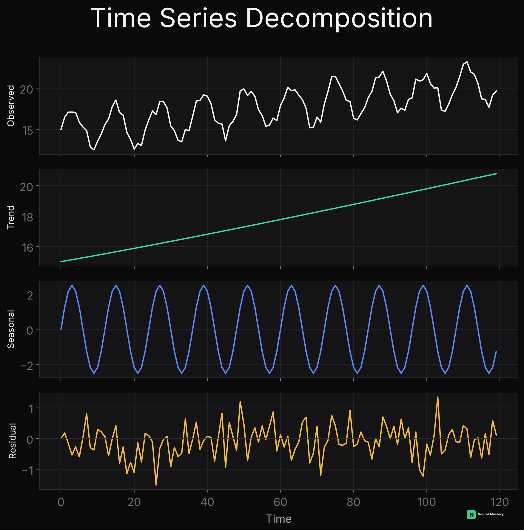
• Trend: the long-run direction — growing, shrinking, flat.
• Seasonal: a pattern that repeats at a fixed, known period (daily, weekly, yearly).
• Residual: whatever's left after removing trend and seasonality — ideally close to random noise; if the residual still has visible structure, the model hasn't captured everything it should.

Classical forecasting models are, in large part, formal ways of modeling these three pieces (or explicitly assuming one away).

ARIMA (AutoRegressive Integrated Moving Average)

ARIMA combines three ideas, named by its three parameters $(p, d, q)$:

• AR($p$) — AutoRegressive: predict the current value as a linear combination of the previous $p$ values: $y_t = c + \phi_1 y_{t-1} + \cdots + \phi_p y_{t-p} + \epsilon_t$. Structurally, this is just linear regression where the "features" are the series' own past values.
• I($d$) — Integrated: apply differencing $d$ times ($y_t' = y_t - y_{t-1}$) before modeling, to remove trend and make the series stationary (statistical properties like mean/variance constant over time — a requirement for AR/MA to work correctly). $d$ is how many times you need to difference before the trend disappears.
• MA($q$) — Moving Average: model the current value as a function of the past $q$ forecast errors, not past values: $y_t = c + \epsilon_t + \theta_1\epsilon_{t-1} + \cdots + \theta_q\epsilon_{t-q}$ — captures short-term shocks whose effect lingers for a few steps before fading.

Real non-stationary series, real differencing applied live:

Choosing $(p,d,q)$: classically done by inspecting ACF (autocorrelation function — correlation between $y_t$ and $y_{t-k}$ across lags $k$) and PACF (partial autocorrelation — the same, controlling for shorter lags) plots, or more commonly today, via automated search (grid search over candidate values, scored by AIC/BIC or cross-validated forecast error — see Model Evaluation & Metrics).

SARIMA: ARIMA + Explicit Seasonality

Plain ARIMA has no dedicated mechanism for seasonality — differencing can remove trend, but a repeating yearly pattern needs its own treatment. SARIMA adds a second, seasonal $(P,D,Q,s)$ set of the exact same AR/I/MA ideas, operating at lag multiples of the seasonal period $s$ (e.g. $s=12$ for monthly data with yearly seasonality) — so the model captures both short-term autocorrelation and the repeating seasonal pattern simultaneously, each with its own order.

Prophet

Facebook/Meta's forecasting library, designed specifically to be robust and usable without deep statistical expertise. Instead of ARIMA's autoregressive structure, Prophet models the series as an explicit additive decomposition:

$y_t = g(t) + s(t) + h(t) + \epsilon_t$

where $g(t)$ is a trend curve (piecewise linear or logistic growth, with automatically-detected changepoints where the trend shifts), $s(t)$ is seasonality modeled via Fourier series (smoothly capturing multiple overlapping seasonal periods — weekly and yearly, simultaneously), and $h(t)$ explicitly accounts for holidays/known special events.

Why teams reach for Prophet over ARIMA: handles missing data and outliers gracefully, requires far less manual tuning of $(p,d,q)$-style orders, and its explicit trend/seasonality/holiday decomposition is directly interpretable — you can plot each component separately and sanity-check it, which is harder with ARIMA's autoregressive coefficients.

The Forecast Output

Regardless of which model, the practical output looks the same: a point forecast plus a widening confidence interval further into the future, reflecting genuinely increasing uncertainty the further out you predict:

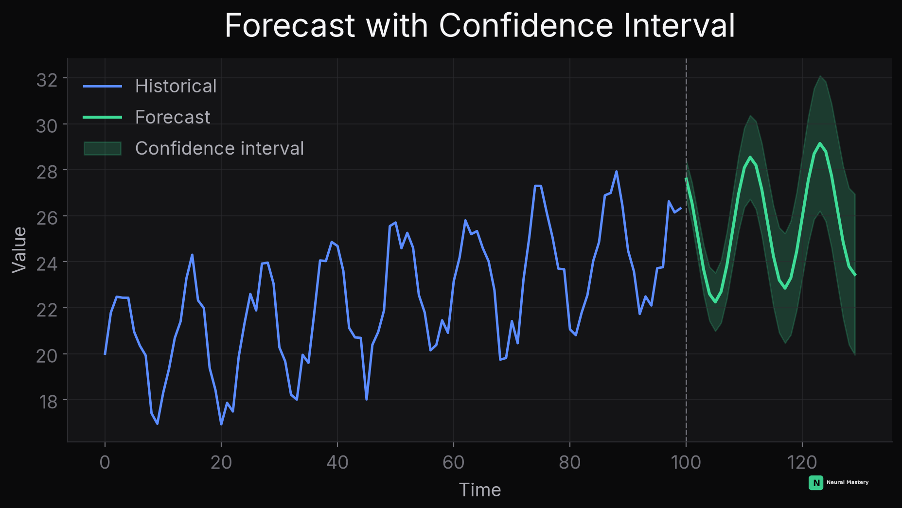
This directly uses Quantile Loss or similar machinery under the hood to produce calibrated upper/lower bounds, not just a single point estimate — critical for any real decision-making use case (inventory planning, capacity planning) where knowing the range of plausible outcomes matters as much as the central estimate.

Temporal Fusion Transformer (TFT)

ARIMA and Prophet fit one model per series, with a fixed, hand-specified structure. TFT is a deep learning approach — it applies attention to forecasting, and can be trained once across many related series simultaneously (e.g. sales for every store in a chain), letting it share learned patterns across them instead of fitting each in isolation.

Its architecture combines several pieces built for this specific problem:

• Variable selection networks: learn which input features actually matter for a given forecast, rather than assuming all inputs are equally relevant — a learned analog of manual feature selection.
• LSTM layers (see Sequence Models) for local, short-term temporal patterns.
• Self-attention (see Attention & Transformers) for long-range dependencies — letting the model directly relate a forecast to a relevant event far in the past, without the information having to pass through every intermediate timestep the way a pure RNN would require.
• Quantile outputs: like Prophet's confidence intervals, TFT directly predicts multiple quantiles (see Loss Functions — Quantile Loss) rather than a single point forecast, giving calibrated uncertainty bounds natively.

When TFT earns its complexity over ARIMA/Prophet: many related series that can share learned structure, rich additional covariates (promotions, weather, holidays) that interact in complex nonlinear ways, and enough data to actually train a deep model well. For a single series with limited data, ARIMA or Prophet usually remains the more practical choice — TFT's flexibility isn't free, and needs enough data to justify it, the same tradeoff as everywhere else deep learning competes with classical methods (see Deep Learning — When to Reach for It).

Evaluating Forecasts

Standard regression metrics (MAE, RMSE) apply, but time series adds one non-negotiable rule: never split train/test randomly. Always split by time — train on the past, test on the future — since evaluating a model on data that came before some of its training data leaks future information backward and produces a wildly over-optimistic result (a direct instance of the data leakage problem, specific to temporal data).

This completes the classical + modern time series forecasting family: ARIMA → SARIMA → Prophet → TFT. Next: Unsupervised Learning — finding structure in data with no target to forecast at all.