Recommender Systems, In Full Depth

"Users who bought this also bought that" is the most commercially valuable prediction problem in applied ML — it's the core of Netflix, Amazon, Spotify, YouTube, and every ad-ranking system, and it blends supervised learning, unsupervised matrix decomposition, and modern deep learning into one problem.

The Core Problem

Given a set of users, a set of items, and some observed interactions (ratings, clicks, purchases), predict which unobserved items a user would like. Two structurally different starting points:

• Content-based filtering: recommend items similar to what a user liked before, based on item features (genre, cast, description embeddings) — works from day one for a new item (no interaction history needed), but tends to over-narrow recommendations to "more of the same" and can't discover a user's latent taste that isn't explainable by stated features.
• Collaborative filtering: recommend based on patterns across many users' behavior — "users similar to you liked this," inferred purely from the interaction matrix, no item content needed at all. Captures latent taste content-based filtering structurally can't, at the cost of the cold-start problem: a brand-new item with zero interactions has nothing to collaborate on.

Most production systems are hybrids, for exactly this complementary-weaknesses reason.

Matrix Factorization

The classical collaborative-filtering workhorse. Represent the user-item interaction matrix $R \in \mathbb{R}^{m \times n}$ (mostly missing entries — no user has rated most items) as the product of two much smaller matrices:

$R \approx U V^T, \quad U \in \mathbb{R}^{m \times k}, \quad V \in \mathbb{R}^{n \times k}$

Each user gets a $k$-dimensional latent factor vector $u_i$, each item gets a $k$-dimensional latent factor vector $v_j$, and the predicted rating is simply their dot product: $\hat{r}_{ij} = u_i \cdot v_j$. $k$ (commonly tens to low hundreds) is far smaller than $m$ or $n$ — the entire method rests on the assumption that user preferences and item characteristics are actually driven by a small number of underlying factors (roughly: genre affinities, price sensitivity, format preference), not by the millions of raw user-item combinations.

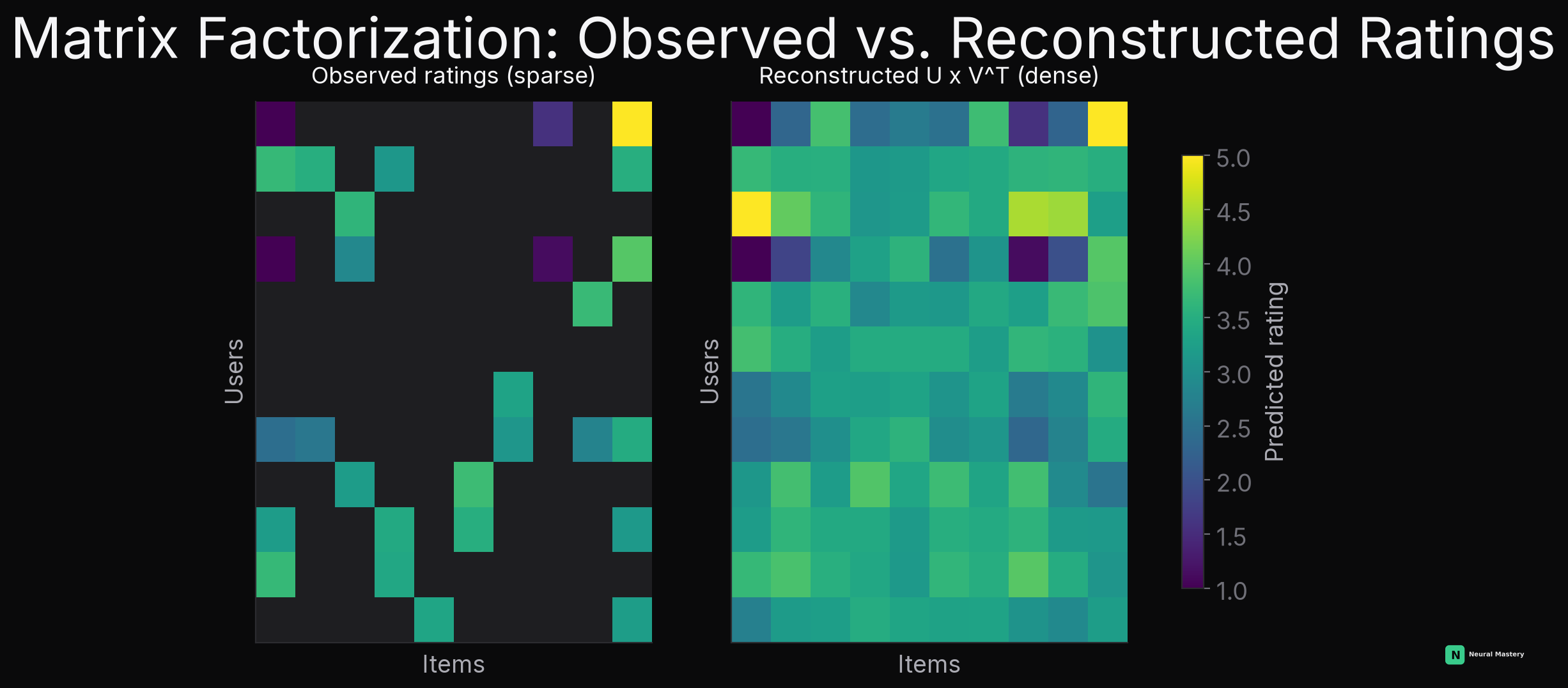
The chart above is exactly this: the left panel is the real, mostly-empty observed data; the right panel is what $UV^T$ predicts for every cell, including the ones that were never observed — that's the entire value of the method, filling in the blanks based on the latent structure learned from the cells that were observed. This is the same low-rank-approximation idea as SVD, applied to a matrix that's sparse (mostly missing) instead of dense. Real gradient descent, trained on only the amber-bordered observed cells below:

Training: minimize squared error over only the observed entries, plus L2 regularization on the factors to prevent overfitting to the (typically very sparse) observed data:

$\min_{U, V} \sum_{(i,j) \in \text{observed}} (r_{ij} - u_i \cdot v_j)^2 + \lambda \left(\|U\|_F^2 + \|V\|_F^2\right)$

Solved via gradient descent, or Alternating Least Squares (ALS) — fix $V$, solve the now-convex problem for $U$ in closed form; fix $U$, solve for $V$; repeat. ALS's appeal is that each half-step is an ordinary (regularized) least-squares problem — the same normal-equations math from Linear Regression — and it parallelizes cleanly across users/items, which is why it was the standard approach at scale for years (Spark's MLlib recommender is ALS).

Embeddings and the Two-Tower Architecture

Modern (deep-learning-based) recommenders generalize matrix factorization's latent vectors into full embeddings — learned dense vectors, but now produced by a neural network from rich features (user history, item metadata, context), not just an ID looked up in a table:

• Two-tower model: one neural network ("tower") encodes user features into a user embedding, a separate tower encodes item features into an item embedding, trained so that the dot product (or cosine similarity) of a user's and item's embeddings is high for real interactions and low otherwise — a direct, learned generalization of $u_i \cdot v_j$ above, now able to incorporate side features and generalize to brand-new users/items whose features are known even without prior interactions (a partial fix for the cold-start problem).
• Why two towers, not one combined network: computing the score for every user-item pair with a single joint network requires re-running the network per pair at serving time — infeasible at real catalog scale. With two separate towers, every item's embedding can be precomputed once and indexed (see Vector Databases), so serving a recommendation becomes a nearest-neighbor search in embedding space — an approximate nearest-neighbor lookup — rather than a forward pass per candidate item.

The Two-Stage Production Pipeline

Real-world recommenders essentially never score the entire catalog for every request — instead:

1. Candidate generation (retrieval): cheaply narrow millions of items down to a few hundred/thousand plausible candidates — typically via the two-tower embedding nearest-neighbor search above, optimized for recall (don't miss good candidates) over precision.
2. Ranking: a much more expensive, feature-rich model (often a gradient-boosted tree or a deep cross-network, incorporating dozens of user/item/context features a lightweight retrieval embedding can't) re-scores and orders just those few hundred candidates precisely, optimized for the actual business metric (predicted CTR, watch time, purchase probability).
3. Re-ranking: business-logic adjustments layered on top of the ranked list — diversity injection (don't show 10 nearly-identical items), freshness boosting, deduplication, and business rules (promoted content, removing already-purchased items) — see Learning-to-Rank for how the ranking stage's model is actually trained.

This funnel shape (cheap-and-broad → expensive-and-narrow) is the standard architecture precisely because it's computationally infeasible to run the expensive ranking model over the full catalog for every request — see ML System Design for the same retrieval-then-rank pattern showing up in search and RAG.

CTR Prediction

Click-Through Rate prediction — will a user click this specific item/ad if shown it — is the ranking-stage model in most ad and feed-ranking systems, framed as binary classification (see Logistic Regression and Boosting) with heavily engineered features: user history aggregates, item popularity, recency, and increasingly, learned embeddings as additional input features alongside hand-engineered ones.

Sequential Recommendation

Instead of treating a user's history as an unordered set of past interactions, model it as a sequence — what a user is likely to want next depends on the order of what they did, not just the set (someone who just bought a phone case probably wants a screen protector next, not "more phones," which a pure collaborative-filtering signal wouldn't naturally distinguish). Architecturally, this reuses the sequence-modeling machinery from Sequence Models and Attention & Transformers directly — a user's interaction history becomes a token sequence, and the "next item" becomes the next-token-prediction target, the same self-attention mechanism that predicts the next word predicting the next likely interaction instead.

Next: Learning-to-Rank — the ranking-stage model training objective in more depth, the same problem sitting underneath recommenders, search, and ad ranking alike.