Decision Trees, In Full Depth

Every model covered so far — Linear, Ridge/Lasso, Logistic Regression — draws a straight (or smoothly curved) boundary through feature space. A decision tree draws something completely different: a sequence of yes/no questions, splitting the data into rectangular regions.

What Is a Decision Tree?

A tree is a nested set of if/else rules learned directly from data, ending in a prediction:

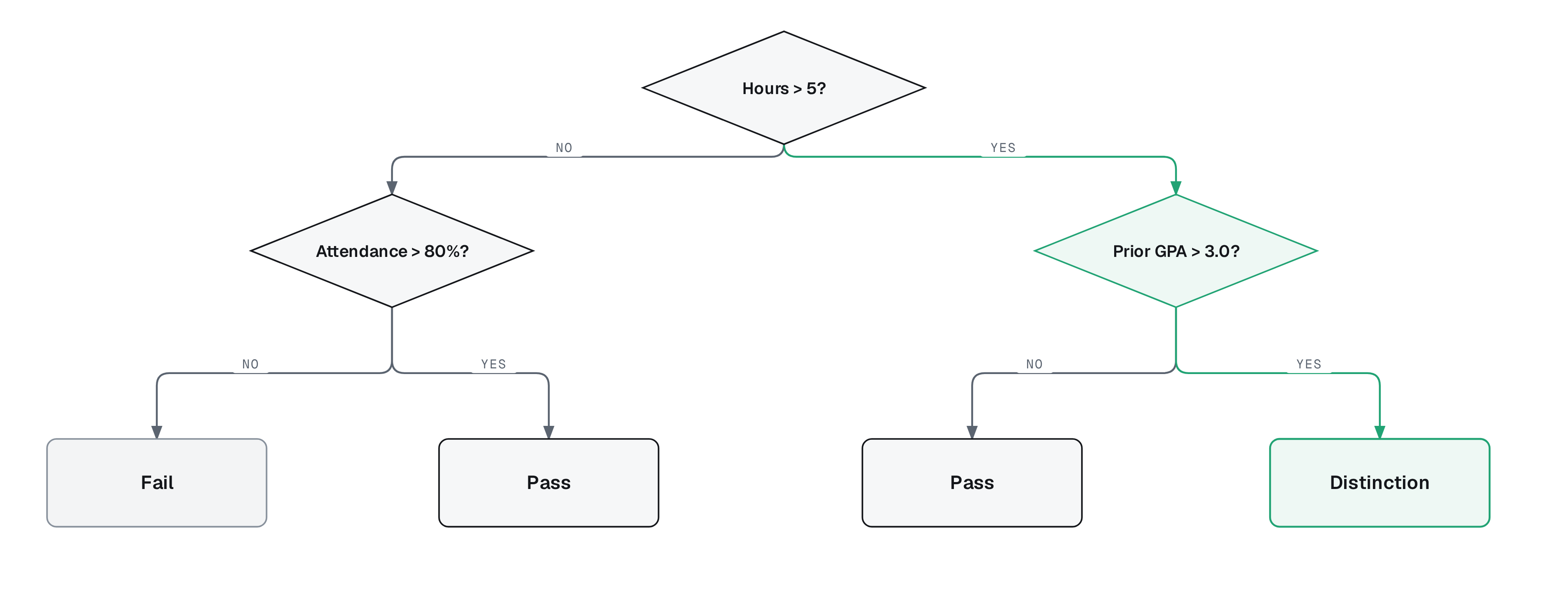
Each internal node asks a single-feature question ("Hours Studied > 5?"), each branch is an answer, and each leaf is a prediction. To predict for a new example, walk down from the root, answering each question, until reaching a leaf.

Why the Boundary Looks Like a Staircase

Because every split tests exactly one feature against a threshold, the resulting decision regions are always axis-aligned rectangles — never diagonal, never curved:

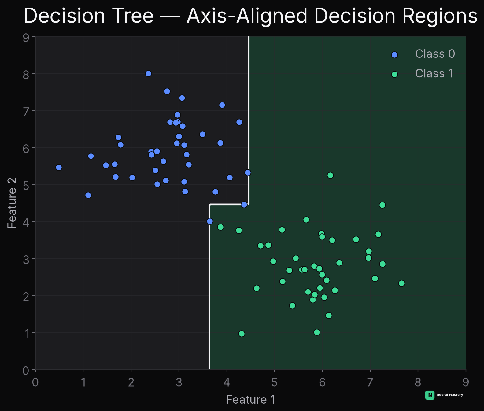
Compare this directly to Logistic Regression's single straight boundary. A tree can carve out any shape given enough splits (it's far more flexible), but that flexibility is exactly why trees overfit so easily — a deep enough tree can wall off every individual training point into its own tiny region, memorizing noise rather than learning a real pattern.

Click to place points and drag Max depth up to watch the staircase get finer — real Gini-impurity splits, computed live:

How a Split Is Chosen

At each node, the tree tries every feature and every possible threshold, and picks whichever split makes the resulting two groups most pure — as unmixed in class labels as possible.

Gini Impurity (classification): $G = 1 - \sum_{c} p_c^2$, where $p_c$ is the fraction of examples in class $c$ at that node. $G=0$ means perfectly pure (one class only); $G$ is maximized when classes are evenly mixed. A split is scored by the weighted average Gini of its two resulting children — lower is better.

Entropy / Information Gain (the alternative criterion): $H = -\sum_c p_c \log_2 p_c$ — the same entropy used throughout information theory. Information gain is the reduction in entropy from parent to children: $IG = H(\text{parent}) - \sum_{\text{child}} \frac{n_{\text{child}}}{n_{\text{parent}}} H(\text{child})$. Gini and entropy nearly always pick similar splits in practice; Gini is slightly cheaper to compute (no logarithm) and is the more common default.

For regression, the criterion switches to variance reduction — minimize the weighted average of each child's variance (equivalently, MSE — see Linear Regression), since there's no "class" to measure impurity over.

The Full Algorithm (Recursive Partitioning)

1. At the current node, try every (feature, threshold) pair; compute the impurity reduction each split would give.
2. Pick the split with the best (largest) impurity reduction.
3. Partition the data into the two children accordingly.
4. Recurse on each child, until a stopping condition: max depth reached, a node is already pure, or too few examples remain to split further.
5. Each final leaf predicts the majority class (classification) or the mean target value (regression) of the training examples that landed there.

This greedy, one-split-at-a-time process is why trees train fast — there's no gradient descent, no iterative optimization loop, just repeated exhaustive search over a shrinking dataset.

Controlling Overfitting

An unconstrained tree will grow until every leaf is perfectly pure — which usually means memorizing the training set. The standard controls:

• Max depth: hard cap on how many questions deep the tree can go.
• Min samples per leaf / per split: refuse to split a node with too few examples, or produce a leaf with too few.
• Min impurity decrease: refuse a split that doesn't improve purity by at least some threshold.
• Pruning: grow the full tree first, then remove branches that don't improve validation performance (see ML Workflow Fundamentals) — a post-hoc alternative to constraining growth upfront.

A single, well-pruned tree is rarely the strongest model on its own — its real value, as the next page covers, is as the building block inside ensembles like Random Forest and Gradient Boosting.

Strengths and Weaknesses

• Interpretable: you can print the tree and read the exact decision logic — hard to match with any other model class.
• No feature scaling needed: splits only compare a feature to a threshold, so scale/units don't matter (unlike Linear Regression or KNN).
• Handles nonlinear relationships and feature interactions natively, unlike plain linear/logistic regression.
• High variance: small changes in training data can produce a completely different tree structure — this instability is exactly what ensembling (next page) fixes.
• Biased toward features with more possible split points (e.g. continuous features over binary ones) unless explicitly corrected.

Minimal Implementation

A single split decision, implementing the Gini criterion directly:

import numpy as np

def gini(y):
    p = np.bincount(y) / len(y)
    return 1 - np.sum(p ** 2)

def best_split(X, y):
    best_feat, best_thresh, best_score = None, None, np.inf
    n_features = X.shape[1]
    for feat in range(n_features):
        for thresh in np.unique(X[:, feat]):
            left = y[X[:, feat] <= thresh]
            right = y[X[:, feat] > thresh]
            if len(left) == 0 or len(right) == 0:
                continue
            weighted_gini = (len(left) * gini(left) + len(right) * gini(right)) / len(y)
            if weighted_gini < best_score:
                best_feat, best_thresh, best_score = feat, thresh, weighted_gini
    return best_feat, best_thresh

Next: Random Forest & Extra Trees — averaging many trees together to fix the single-tree instability problem above.