Naive Bayes, LDA & QDA, In Full Depth

Every classifier so far — logistic regression, SVM, KNN — is discriminative: it learns a boundary directly, without ever modeling what each class's data actually looks like. This page covers the alternative: generative classifiers, which model each class's distribution explicitly, then use Bayes' theorem to classify.

Discriminative vs. Generative

Discriminative models learn $P(y \mid \mathbf{x})$ directly — "given this input, what's the probability of each class?"
Generative models learn $P(\mathbf{x} \mid y)$ for each class — "if this were really class $c$ , what would the data look like?" — plus the class prior $P(y)$ , then combine via Bayes' theorem:

$P(y \mid \mathbf{x}) = \frac{P(\mathbf{x} \mid y)\, P(y)}{P(\mathbf{x})}$

Since $P(\mathbf{x})$ is the same regardless of which class you're evaluating, classification just picks whichever class maximizes the numerator: $\hat{y} = \arg\max_y P(\mathbf{x} \mid y) P(y)$ .

Naive Bayes

The "naive" assumption: features are conditionally independent given the class — $P(\mathbf{x} \mid y) = \prod_j P(x_j \mid y)$ . This is almost never literally true (word co-occurrence in text, correlated pixels in images) — yet Naive Bayes remains a fast, surprisingly strong baseline, especially for text classification, because getting the relative ranking between classes right doesn't actually require the independence assumption to be true, only that violating it doesn't happen to favor the wrong class.

Three variants, differing in what $P(x_j \mid y)$ is assumed to look like:

Gaussian Naive Bayes: assumes each feature is normally distributed within each class — $P(x_j \mid y) = \mathcal{N}(\mu_{j,y}, \sigma_{j,y}^2)$ . The natural choice for continuous features.
Multinomial Naive Bayes: assumes features are counts (e.g. word frequencies in a document) drawn from a multinomial distribution — the standard choice for text classification with bag-of-words features.
Bernoulli Naive Bayes: assumes features are binary (e.g. "does this word appear at all, yes/no") — used for text when only presence/absence matters, not frequency.

Training is just counting: estimate each class's prior $P(y)$ as its frequency in the training set, and each $P(x_j \mid y)$ from the relevant sample statistics (mean/variance for Gaussian, counts for Multinomial/Bernoulli) — no iterative optimization at all, which is exactly why Naive Bayes trains almost instantly even on large datasets.

LDA: Linear Discriminant Analysis

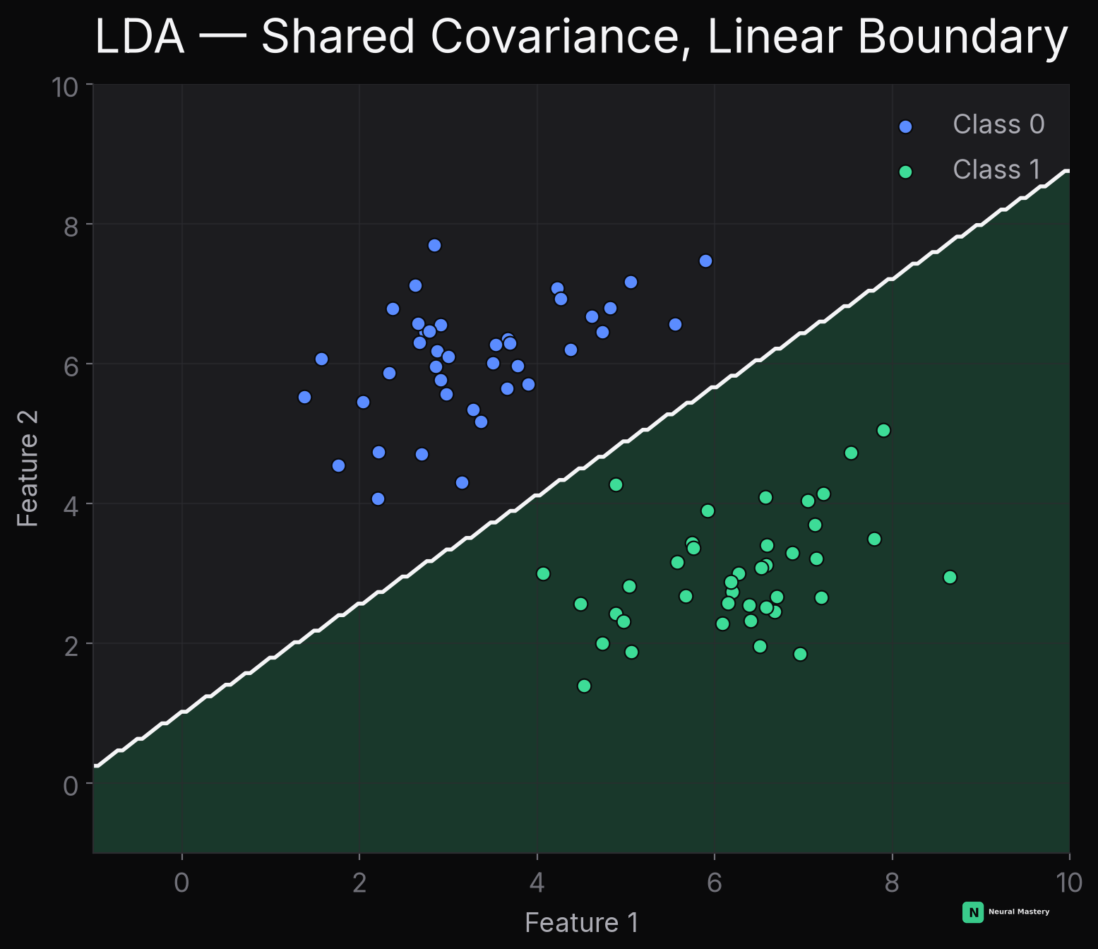
LDA is a specific generative model: assumes each class's features follow a multivariate Gaussian, and — critically — that every class shares the same covariance matrix $\Sigma$ , differing only in their means $\mu_y$ .

Under this assumption, the log-ratio $\log\frac{P(y=1\mid\mathbf{x})}{P(y=0\mid\mathbf{x})}$ works out to be linear in $\mathbf{x}$ — the quadratic terms from the Gaussian density cancel exactly because both classes share the same $\Sigma$ . That's why LDA produces a straight-line boundary:

LDA's decision boundary is exactly linear, because both classes share the same covariance shape

QDA: Quadratic Discriminant Analysis

Drop LDA's shared-covariance assumption — let each class have its own covariance matrix $\Sigma_y$ . Now the quadratic terms in the log-ratio no longer cancel, producing a genuinely curved boundary:

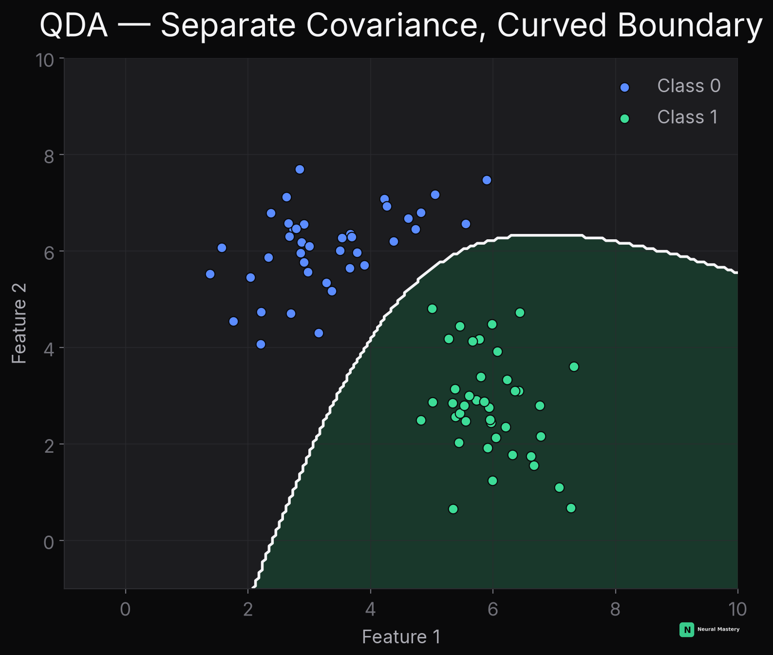
QDA's decision boundary curves, because each class now has its own covariance shape

Toggle between the two directly on the same real data, with each boundary computed live from real fitted means and covariances rather than pre-rendered:

Model

Real decision boundary = the shading transition, computed from each model's actual discriminant score at every grid point, not drawn by hand.

Real fitted Gaussians from the 120 points below. QDA fits each class its own real covariance matrix -- since class 1 is genuinely more spread out along x than class 0, the real boundary curves to follow that actual difference in shape.

LDA vs. QDA

More flexible isn't automatically better — QDA has far more parameters to estimate (a full covariance matrix per class instead of one shared matrix), so it needs proportionally more data to estimate them reliably. With limited data, LDA's extra assumption acts as a form of regularization: it accepts a bit more bias (forcing a linear boundary even if the true boundary curves slightly) in exchange for much lower variance in the estimated parameters. The same bias-variance tradeoff appears here as everywhere else in this curriculum (Model Evaluation & Metrics) — just expressed through a modeling assumption instead of a regularization hyperparameter.

Naive Bayes vs. LDA vs. QDA

	Naive Bayes	LDA	QDA
Feature independence assumed?	Yes	No (models full covariance)	No
Covariance shared across classes?	N/A (independent features)	Yes	No, per-class
Boundary shape	Depends on distribution choice	Linear	Quadratic (curved)
Parameters to estimate	Fewest	Moderate	Most
Best when	Many features, limited data (esp. text)	Gaussian-ish classes, similar spread	Gaussian-ish classes, genuinely different spread per class

Minimal Implementation

Gaussian Naive Bayes, matching the derivation above directly:

import numpy as np

def fit_gaussian_nb(X, y):
    classes = np.unique(y)
    params = {}
    for c in classes:
        X_c = X[y == c]
        params[c] = {
            "mean": X_c.mean(axis=0),
            "var": X_c.var(axis=0) + 1e-9,
            "prior": len(X_c) / len(X),
        }
    return params

def predict_gaussian_nb(X, params):
    log_probs = []
    for c, p in params.items():
        log_likelihood = -0.5 * np.sum(
            np.log(2 * np.pi * p["var"]) + (X - p["mean"]) ** 2 / p["var"], axis=1
        )
        log_probs.append(np.log(p["prior"]) + log_likelihood)
    log_probs = np.array(log_probs)
    classes = list(params.keys())
    return np.array([classes[i] for i in log_probs.argmax(axis=0)])

Next: SGD Classifier & Regressor — the generic "any linear model, trained via SGD" framing that ties the linear-model family together.