ICA, t-SNE & UMAP, In Full Depth
PCA and its relatives all optimize for variance. This page covers three methods with a different goal entirely: ICA separates mixed signals by statistical independence, while t-SNE and UMAP optimize purely to make high-dimensional data visualizable, with no interest in variance or interpretable axes at all.
Independent Component Analysis (ICA)
The classic motivating example — the "cocktail party problem": imagine several microphones in a room with several people talking simultaneously. Each microphone records a different mixture of all the voices. ICA's job: given only the mixed recordings, recover the original, separate voices.
The key assumption: unlike PCA (which looks for directions of maximum variance, and produces components that are merely uncorrelated), ICA looks for components that are statistically independent — a much stronger condition. Two variables can be uncorrelated (zero linear relationship) while still being highly dependent in a nonlinear way; independence rules out any relationship, linear or not.
Why independence, and why it works: ICA relies on the Central Limit Theorem (see Probability & Statistics) in reverse — a mixture of independent signals tends to look more Gaussian than any of the original signals alone (sums of independent random variables trend toward Gaussian). So ICA searches for a transformation that makes the resulting components as non-Gaussian as possible, on the logic that this is exactly what un-mixes the original signals back out. Real signals, a real linear mixing matrix, and real non-Gaussianity (excess kurtosis) measured before and after:
Practical uses beyond audio: separating overlapping sources in EEG/fMRI brain signal data, removing specific artifacts (like eye-blink noise) from a signal, and general blind source separation problems — anywhere the data is genuinely a mixture of independent underlying causes, which is a different situation than PCA's "compress correlated features" use case.
t-SNE (t-Distributed Stochastic Neighbor Embedding)
Built for exactly one job: taking high-dimensional data (like embeddings — see Foundation Model Internals) and projecting it into 2D/3D purely for visualization, preserving local neighborhood structure as faithfully as possible.
The mechanism: for every pair of points, compute a probability that one would "pick" the other as a neighbor, based on distance in the original high-dimensional space (closer points get higher probability — using a Gaussian kernel). Then, place points in the low-dimensional space and adjust their positions so the same neighbor-probabilities (this time using a heavier-tailed t-distribution, which is where the "t" comes from) match as closely as possible.
The heavy-tailed trick, specifically: using a t-distribution (rather than Gaussian) in the low-dimensional space deliberately allows moderately-distant points to end up farther apart than they'd naturally be — this directly combats the "crowding problem," where high-dimensional space simply has more room than 2D/3D, so naively squashing it down would crush everything into an undifferentiated blob.
Critical caveats — the most commonly misread output in this entire curriculum:
- Cluster sizes in a t-SNE plot are meaningless. A tight-looking cluster and a spread-out one may represent equally tight groupings in the true high-dimensional space — t-SNE doesn't preserve density.
- Distances between separate clusters are meaningless. Two clusters that look close together in the 2D plot are not necessarily more similar than two that look far apart — t-SNE only tries to preserve local neighbor relationships, not global distances.
- Results depend heavily on the perplexity hyperparameter (roughly, the assumed number of effective neighbors) — different values can produce visibly different-looking plots from the same data.
UMAP (Uniform Manifold Approximation and Projection)
Solves the same visualization problem as t-SNE, built on different mathematical foundations (topology and manifold learning rather than t-SNE's probability-matching), but the practical differences are what matter:
- Much faster, especially on large datasets — scales notably better than t-SNE.
- Better preserves global structure — the relative positioning of distinct clusters is more meaningful in UMAP than in t-SNE, though still not fully reliable for precise distance comparisons.
- Can be used for general-purpose dimensionality reduction, not just 2D/3D visualization (t-SNE is rarely used beyond visualization).
In practice: UMAP has largely replaced t-SNE as the default choice for visualizing embeddings and high-dimensional clusters, mainly for the speed advantage on large modern datasets — though both remain in active use, and the same misreading caveats above apply to UMAP's cluster sizes and distances too.
What a Good Embedding Visualization Looks Like
Regardless of method, a successful 2D projection of well-separated high-dimensional categories should show visually distinct groups:
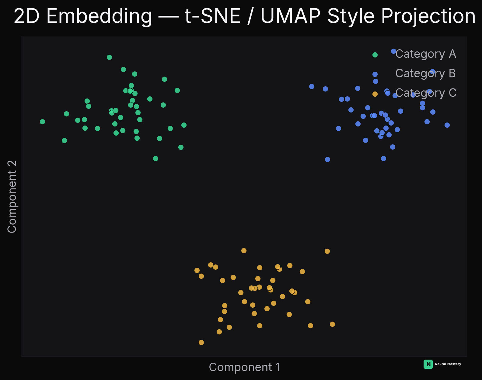
This is exactly the kind of plot you'd generate to sanity-check a trained embedding model (see RAG — Choosing an Embedding Model): project a sample of embeddings to 2D and visually confirm that semantically different categories actually separate, before trusting the embedding space for retrieval.
Choosing Among Dimensionality Reduction Methods
| PCA/SVD | Kernel PCA | ICA | t-SNE | UMAP | |
|---|---|---|---|---|---|
| Goal | Max variance | Nonlinear max variance | Statistical independence | Local structure for visualization | Local + some global structure |
| Linear? | Yes | No | Yes (linear un-mixing) | No | No |
| Deterministic? | Yes | Yes | Mostly | No (random init) | Mostly |
| Good for general compression? | Yes | Sometimes | No (specific use case) | No | Somewhat |
| Good for visualization? | Basic | Rarely used for this | No | Yes (gold standard) | Yes (faster, more scalable) |
This completes dimensionality reduction: PCA/Kernel PCA/Truncated SVD → ICA/t-SNE/UMAP. Next: Anomaly Detection and the remaining unsupervised methods — association rule mining and autoencoders.