Logistic Regression, In Full Depth

Despite the name, logistic regression is a classification algorithm, not a regression one — it predicts a probability, then a class. It's the natural next step after Linear Regression: same linear core, adapted to output something that behaves like a probability.

What Is Logistic Regression?

Linear regression predicts an unbounded real number. That's wrong for classification — if you're predicting "is this email spam?", you want an output between 0 and 1 that behaves like a probability, not a number that could be -40 or +1000.

Logistic regression fixes this with one change: take the linear regression output and squash it through the sigmoid function.

Same study-hours story as Linear Regression, now predicting pass/fail instead of a score. Drag $w$ and $b$ and watch the sigmoid curve — and the accuracy — respond live:

The Sigmoid Function

$\sigma(z) = \frac{1}{1 + e^{-z}}, \qquad z = \mathbf{w}^T\mathbf{x} + b$

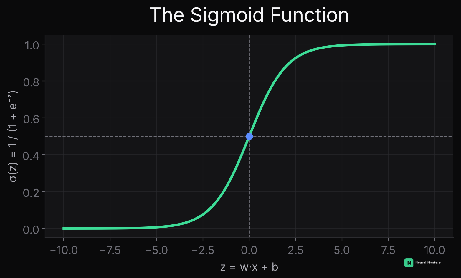
Read directly off the curve: as $z \to +\infty$, $\sigma(z) \to 1$; as $z \to -\infty$, $\sigma(z) \to 0$; at $z=0$, $\sigma(z) = 0.5$ exactly. No matter what real number $z = \mathbf{w}^T\mathbf{x}+b$ comes out of the linear part, $\sigma(z)$ always lands in $(0,1)$ — a valid probability. The full hypothesis:

$\hat{p} = \sigma(\mathbf{w}^T\mathbf{x} + b)$

$\hat{p}$ is interpreted as $P(y=1 \mid \mathbf{x})$. To get an actual class prediction, threshold it — conventionally $\hat{y} = 1$ if $\hat{p} \geq 0.5$, else $\hat{y} = 0$ (equivalently: predict class 1 whenever $z \geq 0$).

Try it yourself: implement the sigmoid activation from scratch, against real test cases.

Why Not Just Use MSE Loss?

You could plug $\hat{p}$ into the same MSE cost function from linear regression. It would technically run — but the resulting cost surface is non-convex in $(\mathbf{w}, b)$ when combined with the sigmoid, full of local minima that gradient descent can get stuck in. Logistic regression uses a different loss specifically chosen to stay convex.

Don't take that on faith — switch the Studio above to Gradient Descent Lab mode and toggle the Loss function between Cross-Entropy and MSE (naive). Both start from the same deliberately bad initialization: Cross-Entropy steadily escapes it; MSE-on-sigmoid gets stuck almost immediately and barely moves for hundreds of steps — the loss landscape panel shows exactly why: a visibly bumpier, flatter-near-the-wrong-answer surface instead of cross-entropy's clean bowl.

The Cost Function: Binary Cross-Entropy

$J(\mathbf{w}, b) = -\frac{1}{n}\sum_{i=1}^n \left[y^{(i)}\log(\hat{p}^{(i)}) + (1-y^{(i)})\log(1-\hat{p}^{(i)})\right]$

This looks intimidating but is simple per-example: only one of the two terms is ever "active," because $y^{(i)}$ is either 0 or 1.

• If $y^{(i)} = 1$: the second term vanishes ($1-y^{(i)}=0$), leaving $-\log(\hat{p}^{(i)})$. This is small when $\hat{p}^{(i)}$ is close to 1 (correct, confident) and blows up toward $+\infty$ as $\hat{p}^{(i)} \to 0$ (confidently wrong) — exactly the penalty behavior you want.
• If $y^{(i)} = 0$: the first term vanishes, leaving $-\log(1-\hat{p}^{(i)})$ — small when $\hat{p}^{(i)}$ is close to 0, blowing up as $\hat{p}^{(i)} \to 1$.

This is exactly cross-entropy from Probability & Statistics, specialized to two classes — and it's not an arbitrary design choice: minimizing this loss is precisely Maximum Likelihood Estimation for a Bernoulli-distributed target (see MLE vs MAP). Unlike MSE-on-sigmoid, this cost function is convex in $(\mathbf{w}, b)$, so gradient descent is guaranteed to find the global minimum.

Deriving the Gradient

This is where something elegant happens. Working through the chain rule — differentiating the log-loss with respect to $z$, then $z$ with respect to $w_j$ — the sigmoid's own derivative ($\sigma'(z) = \sigma(z)(1-\sigma(z))$) cancels almost entirely against terms from the log-loss derivative, leaving:

$\frac{\partial J}{\partial w_j} = \frac{1}{n}\sum_{i=1}^n \left(\hat{p}^{(i)} - y^{(i)}\right)x_j^{(i)}$

This is the identical formula shape as linear regression's gradient (see Linear Regression — Section 3) — "error times input," summed over examples — even though the loss function and the model's output are completely different. This isn't a coincidence: it's a general property of combining a sigmoid/softmax output with cross-entropy loss (the same clean gradient shape reappears in neural network classifiers and in LLM next-token prediction).

The gradient descent update is then identical in form to linear regression's:

$w_j \leftarrow w_j - \alpha \cdot \frac{1}{n}\sum_i \left(\hat{p}^{(i)} - y^{(i)}\right)x_j^{(i)}$

The Decision Boundary

Because $z = \mathbf{w}^T\mathbf{x}+b$ is linear, and the threshold is at $z=0$, the boundary between predicted classes is a straight line (or a flat hyperplane in higher dimensions):

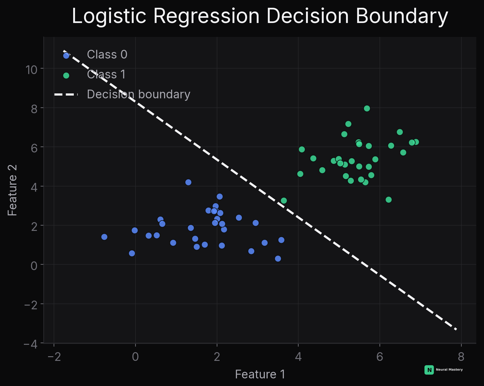
This is the central limitation of plain logistic regression: it can only separate classes that are (approximately) linearly separable. Data that needs a curved boundary requires either engineered polynomial features, or a fundamentally different model (see SVM with a kernel, or a neural network).

Regularized Logistic Regression

Exactly like linear regression, logistic regression overfits with too many features relative to data — and the same fix applies directly: add an L2 (or L1) penalty to $J(\mathbf{w}, b)$ above, identical in form to Ridge or Lasso's penalty term. This is in fact the default behavior in most libraries (e.g. scikit-learn regularizes logistic regression by default) — unregularized logistic regression is the exception, not the norm, in practice.

Multi-Class: Softmax Regression

For more than two classes, the sigmoid generalizes to the softmax function, and binary cross-entropy generalizes to categorical cross-entropy — the exact loss used to train every classifier's output layer in Deep Learning, including next-token prediction in every LLM (see Training Pipeline).

Try it yourself: implement a numerically stable softmax from scratch, against real test cases.

Minimal Implementation

import numpy as np

def sigmoid(z):
    return 1 / (1 + np.exp(-z))

def fit_logistic_regression(X, y, lr=0.1, epochs=1000):
    n, d = X.shape
    w = np.zeros(d)
    b = 0.0
    for _ in range(epochs):
        z = X @ w + b
        p_hat = sigmoid(z)
        error = p_hat - y                   # identical shape to linear regression's gradient
        dw = (1 / n) * X.T @ error
        db = (1 / n) * np.sum(error)
        w -= lr * dw
        b -= lr * db
    return w, b

def predict(X, w, b, threshold=0.5):
    return (sigmoid(X @ w + b) >= threshold).astype(int)

Next: Model Evaluation & Metrics for precision/recall/ROC-AUC — the metrics that actually matter for judging a classifier, since accuracy alone is misleading on imbalanced data.