Ridge Regression, In Full Depth

Ordinary linear regression (see Linear Regression) has a failure mode: when features are highly correlated, or there are more features than examples, $(X^TX)^{-1}$ becomes unstable — small changes in the data cause huge swings in the fitted weights. Ridge regression fixes this by penalizing large weights directly in the loss function.

What Is Ridge Regression?

Ridge is linear regression with one addition: a penalty term that discourages weights from growing large. The hypothesis is identical to plain linear regression — $\hat{y} = \mathbf{w}^T\mathbf{x} + b$ — only the cost function changes.

Why penalize large weights at all? A model with huge, wildly-swinging coefficients has usually latched onto noise in the training data rather than a real signal — a hallmark of overfitting (see Model Evaluation & Metrics — Bias-Variance Tradeoff). Shrinking the weights trades a small amount of bias for a large reduction in variance, which usually wins on unseen data.

The Ridge Cost Function

$J_{\text{ridge}}(\mathbf{w}, b) = \underbrace{\frac{1}{n}\sum_{i=1}^n \left(\hat{y}^{(i)} - y^{(i)}\right)^2}_{\text{same MSE as OLS}} + \underbrace{\lambda \sum_{j=1}^d w_j^2}_{\text{L2 penalty}}$

The first term is exactly the MSE cost function from plain linear regression. The second term — $\lambda \sum w_j^2$, the squared L2 norm of the weight vector (see Linear Algebra — Norms) — is new. $\lambda \geq 0$ controls the tradeoff: $\lambda = 0$ recovers plain OLS exactly; larger $\lambda$ shrinks weights more aggressively toward zero. Note the bias $b$ is not penalized — only shrinking the feature weights makes sense, since $b$ just sets the overall output level.

Deriving the Gradient

The MSE part of the gradient is unchanged from Linear Regression — Section 3. The new penalty term adds $\frac{\partial}{\partial w_j}\left(\lambda w_j^2\right) = 2\lambda w_j$:

$\frac{\partial J_{\text{ridge}}}{\partial w_j} = \underbrace{\frac{2}{n}\sum_{i=1}^n \left(\hat{y}^{(i)} - y^{(i)}\right) x_j^{(i)}}_{\text{OLS gradient}} + 2\lambda w_j$

The gradient descent update becomes:

$w_j \leftarrow w_j - \alpha\left(\frac{2}{n}\sum_i \left(\hat{y}^{(i)} - y^{(i)}\right)x_j^{(i)} + 2\lambda w_j\right) = w_j(1 - 2\alpha\lambda) - \alpha \cdot (\text{OLS gradient term})$

Written this way, the mechanism is obvious: every single update step first shrinks $w_j$ by a factor of $(1 - 2\alpha\lambda)$ before applying the usual OLS correction. This is why ridge is sometimes called "weight decay" in the deep learning literature (see Training Deep Networks — Regularization) — it's the exact same mechanism.

The Closed-Form Solution

Ridge has a closed form too, a small modification of the normal equation:

$\mathbf{w} = (X^TX + \lambda I)^{-1}X^T\mathbf{y}$

This is why ridge regression exists mathematically, not just statistically: adding $\lambda I$ to $X^TX$ before inverting guarantees the matrix is invertible, even when $X^TX$ alone is singular or near-singular (highly correlated features, or more features than examples). Plain OLS can fail outright in that situation; ridge never does, for any $\lambda > 0$.

The Regularization Path

As $\lambda$ increases from 0, every weight shrinks smoothly toward zero — but critically, never exactly reaches zero (except in the limit $\lambda \to \infty$):

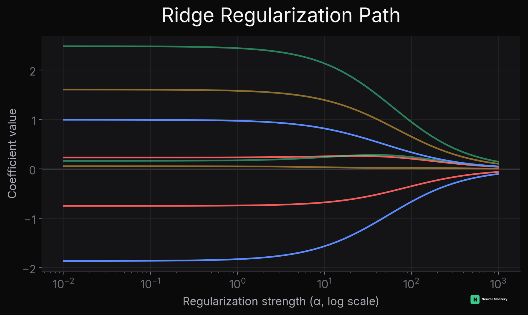
Compare this to Lasso's path — the visual difference between the two curves is the core conceptual difference between L2 and L1 regularization.

Try it on a real (small, synthetic) multicollinear dataset — drag $\lambda$ from 0 and watch two deliberately correlated features fight over shared credit, then settle down:

Choosing λ

$\lambda$ is a hyperparameter, not learned from the training data directly — it's chosen via cross-validation (see ML Workflow Fundamentals): train with several candidate $\lambda$ values, and pick whichever generalizes best on a held-out validation set.

When to Use Ridge

• Many correlated features (ridge handles multicollinearity gracefully — plain OLS coefficients become unstable, ridge's don't)
• More features than examples, or close to it
• You want to keep all features in the model, just with controlled magnitude (contrast with Lasso, which drops features entirely)

Minimal Implementation

import numpy as np

def fit_ridge(X, y, lam=1.0, lr=0.01, epochs=1000):
    n, d = X.shape
    w = np.zeros(d)
    b = 0.0
    for _ in range(epochs):
        y_hat = X @ w + b
        error = y_hat - y
        dw = (2 / n) * X.T @ error + 2 * lam * w   # OLS gradient + ridge penalty
        db = (2 / n) * np.sum(error)                # bias is never penalized
        w -= lr * dw
        b -= lr * db
    return w, b

# Closed form, for comparison
def fit_ridge_normal_equation(X, y, lam=1.0):
    d = X.shape[1]
    return np.linalg.inv(X.T @ X + lam * np.eye(d)) @ X.T @ y

Next: Lasso Regression — the L1 alternative that drops features entirely instead of just shrinking them.