Support Vector Machines (SVM & SVR), In Full Depth

Logistic Regression finds a line that separates classes. SVM finds the line that separates them with the widest possible gap — a subtly different objective that turns out to have far-reaching consequences.

What Is an SVM?

Given linearly separable data, there are infinitely many lines that correctly separate the two classes. SVM picks the one that maximizes the margin — the distance from the boundary to the nearest point of either class:

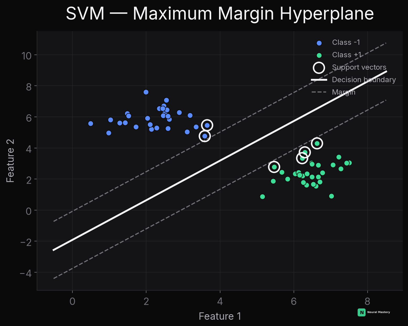
Why maximize the margin specifically? Intuitively, a boundary that barely squeezes between the classes is fragile — a new point close to the boundary could easily land on the wrong side. A wide-margin boundary is the most "confident" separator possible, and this intuition has a rigorous backing: maximum-margin classifiers have provably better generalization bounds than arbitrary separating hyperplanes.

Support Vectors

The margin is defined entirely by the points closest to the boundary — the support vectors (circled above). Every other point could move anywhere further from the boundary without changing the solution at all. This is SVM's defining structural property: the model is determined by a small subset of the training data, not by all of it — contrast this with Linear Regression, where every single point pulls on the fitted line via the MSE gradient.

The Optimization Problem

Maximize margin $= \frac{2}{\|\mathbf{w}\|}$ subject to every point being correctly classified with margin at least 1: $y_i(\mathbf{w}^T\mathbf{x}_i + b) \geq 1$ for all $i$ . Maximizing $\frac{2}{\|\mathbf{w}\|}$ is equivalent to minimizing $\|\mathbf{w}\|^2$ — so the problem becomes:

$\min_{\mathbf{w}, b} \frac{1}{2}\|\mathbf{w}\|^2 \quad \text{subject to} \quad y_i(\mathbf{w}^T\mathbf{x}_i + b) \geq 1 \;\, \forall i$

This is a quadratic program — a convex optimization problem (see Calculus & Optimization — Convexity) with linear constraints, solvable exactly (no gradient descent required, though it can also be solved that way in practice).

Soft Margin: Handling Non-Separable Data

Real data is rarely perfectly separable. The soft margin SVM allows some points to violate the margin (or even end up on the wrong side), at a cost:

$\min_{\mathbf{w},b} \frac{1}{2}\|\mathbf{w}\|^2 + C\sum_i \max(0,\ 1 - y_i(\mathbf{w}^T\mathbf{x}_i+b))$

The second term is exactly Hinge Loss — zero once a point is correctly classified with sufficient margin, growing linearly for violations. $C$ controls the tradeoff: large $C$ heavily penalizes margin violations (narrower margin, less tolerant of misclassification — can overfit); small $C$ tolerates more violations for a wider, more robust margin (can underfit). This is the SVM's direct analog of the regularization strength $\lambda$ in Ridge/Lasso.

The Kernel Trick

SVM as described so far only draws straight lines. The kernel trick is what lets it handle non-linear boundaries, and the idea is genuinely elegant: the optimization problem above only ever needs dot products between pairs of points, $\mathbf{x}_i \cdot \mathbf{x}_j$ — never the raw feature vectors individually. So replace that dot product with a kernel function $K(\mathbf{x}_i, \mathbf{x}_j)$ that computes the dot product as if the points had been mapped into some higher-dimensional space first — without ever actually computing that mapping.

Linear kernel: $K(\mathbf{x}_i,\mathbf{x}_j) = \mathbf{x}_i \cdot \mathbf{x}_j$ — the plain SVM above.
Polynomial kernel: $K(\mathbf{x}_i,\mathbf{x}_j) = (\mathbf{x}_i \cdot \mathbf{x}_j + c)^d$ — equivalent to adding polynomial feature combinations, without explicitly constructing them.
RBF (Gaussian) kernel: $K(\mathbf{x}_i,\mathbf{x}_j) = \exp(-\gamma\|\mathbf{x}_i - \mathbf{x}_j\|^2)$ — implicitly corresponds to an infinite-dimensional feature space. The most common default for non-linear SVM, with $\gamma$ controlling how far each point's influence reaches.

This is why SVMs were historically so powerful for non-linear problems before deep learning: full non-linear modeling power, without ever paying the computational cost of actually working in a high (or infinite) dimensional space. A real, minimal example of the underlying idea — real data, genuinely not linearly separable in 1D, made separable by an explicit feature map:

1D: not linearly separable

2D via φ(x) = (x, x²): linearly separable

Real x² values plotted, real separating line drawn where the classes actually split (y=1.7) -- not illustrative placeholders.

No 1D threshold can separate these two classes -- the positive class sits on both ends. Map every point x to (x, x²) -- a real, explicit feature map -- and a single straight line separates them perfectly in 2D. A kernel computes the DOT PRODUCT this mapping would produce, without ever materializing the higher-dimensional coordinates, which is what makes this trick work even when the implied space is infinite-dimensional (RBF kernel).

SVR: Support Vector Regression

The same margin idea, adapted for regression: instead of finding a boundary that separates classes with maximum margin, SVR fits a function such that as many points as possible fall within an $\epsilon$ -wide tube around it, and only penalizes points outside that tube (again via a hinge-like loss). Points strictly inside the tube contribute nothing to the loss at all — a form of built-in tolerance for small errors, unlike MSE, which penalizes every deviation no matter how small.

When to Use SVM

Effective in high-dimensional spaces, even when the number of features exceeds the number of examples.
Memory-efficient at inference (only support vectors matter).
Doesn't scale well to very large datasets — training is at least quadratic in the number of examples for standard solvers, far worse than logistic regression or tree-based methods at scale.
Mostly superseded by gradient-boosted trees (XGBoost/LightGBM/CatBoost) for tabular data and by deep learning for unstructured data — but still a strong choice for smaller, high-dimensional problems (e.g. text classification with TF-IDF features).

Next: K-Nearest Neighbors — a completely different philosophy: no training phase, no learned boundary at all.