Survival Analysis: Kaplan-Meier & Cox Proportional Hazards, In Full Depth

"How long until this happens" is a different prediction problem from "will this happen" — and a subtler one than it first looks, because in almost every real dataset, some subjects haven't experienced the event yet by the time you have to analyze the data. Survival analysis is the branch of statistics/ML built specifically to handle that.

The Core Problem: Censoring

A survival analysis dataset records, for each subject, a time and an event indicator: did the event of interest (death, churn, failure, default) happen, and if so, when? The complication that makes this its own field rather than plain regression is censoring:

• Right-censoring: the most common case — a subject hasn't experienced the event by the end of the observation window (a customer is still active when the study ends; a patient is still alive at the last follow-up). You know they survived at least that long, but not their actual event time.
• Treating censored subjects as "no event" (a naive classification framing) throws away real information (they did survive that long) and biases estimates toward shorter survival times. Treating them as if they experienced the event at the censoring time is equally wrong in the other direction. Survival analysis handles this correctly by using every subject's observed time — event or censored — in the likelihood, without pretending to know what happens after censoring.

Where this shows up outside medicine: customer churn (a still-subscribed customer is right-censored, not "will never churn"), equipment/component failure prediction, time-to-conversion in marketing, employee attrition, loan default timing — anywhere "time until X" matters and X hasn't happened for everyone in the dataset yet.

The Survival Function

$S(t) = P(T > t)$

The probability a subject survives past time $t$. $S(0) = 1$ (everyone starts "alive"), and $S(t)$ decreases monotonically as $t$ grows. Nearly everything in this page is about estimating $S(t)$ well, or modeling how covariates shift it.

The Kaplan-Meier Estimator

The Kaplan-Meier estimator computes $S(t)$ directly from data, non-parametrically — no assumption about the shape of the underlying distribution, just the observed event and censoring times:

$\hat{S}(t) = \prod_{t_i \leq t} \left(1 - \frac{d_i}{n_i}\right)$

At each observed event time $t_i$: $n_i$ is the number of subjects still "at risk" (not yet censored or experienced the event) just before $t_i$, and $d_i$ is the number of events that happened exactly at $t_i$. The estimator is a product of conditional survival probabilities — "survived past each event time, given you'd survived to just before it" — which is exactly why the curve is a step function that only drops at observed event times, and why censored subjects still contribute (they count in $n_i$ for every event time up to their censoring time, then drop out of the risk set without ever contributing a $d_i$).

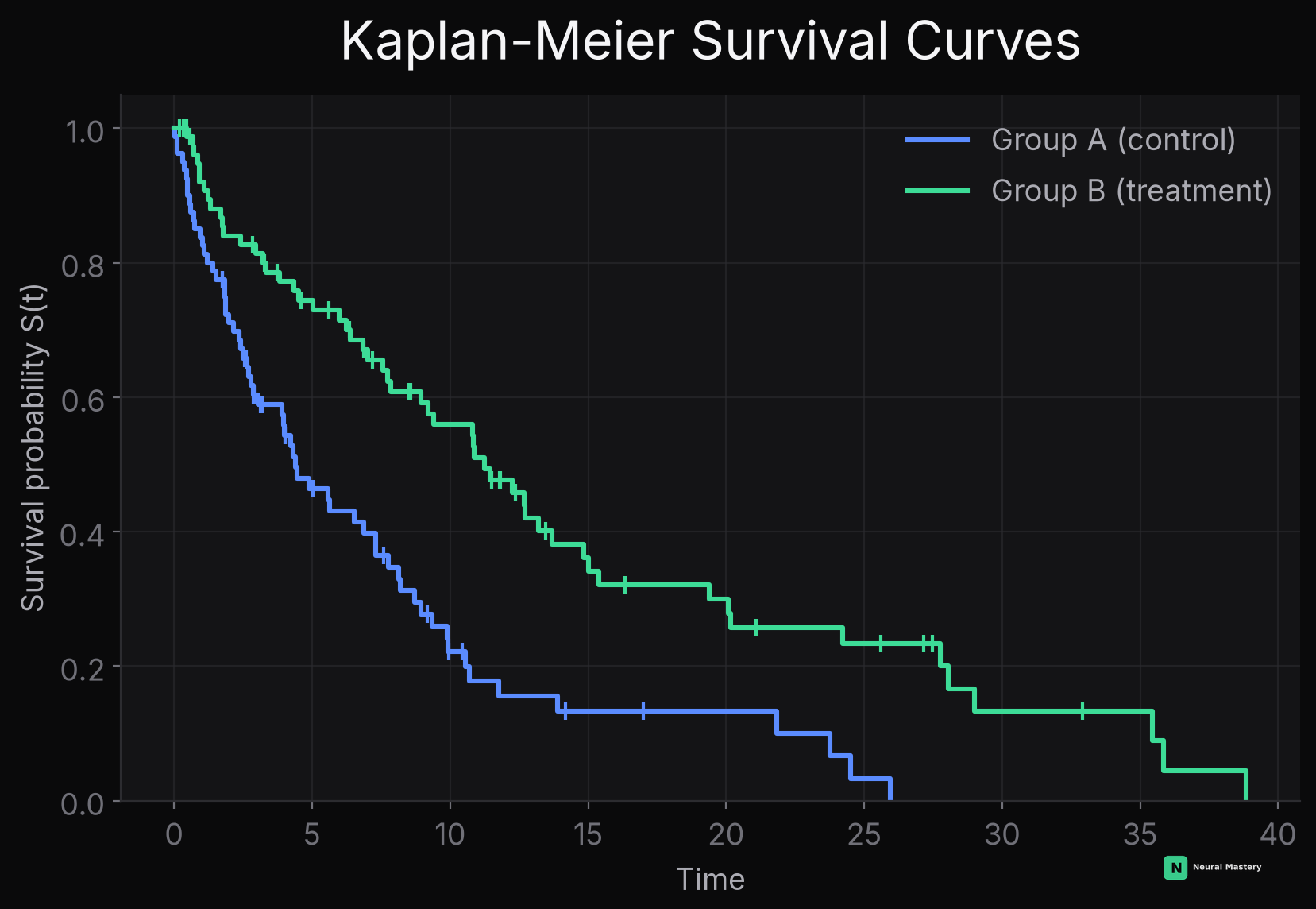
The chart above shows exactly this: each step down is an event, each tick mark is a censored subject leaving the risk set without an event. Group B's curve staying higher for longer is the direct visual read of "this group survives longer" — the entire point of plotting $\hat{S}(t)$ instead of reporting a single summary number.

Step through the real product formula, one real event time at a time, on a real 10-subject toy dataset:

Comparing Groups: The Log-Rank Test

To test whether two Kaplan-Meier curves are significantly different (not just visibly different, per Hypothesis Testing), the log-rank test compares the observed number of events in each group, at each event time, against the number expected if both groups actually had identical survival — summed into a single chi-squared test statistic across all event times. This is the standard significance test reported alongside a Kaplan-Meier plot in a clinical trial or an A/B-style churn comparison.

The Cox Proportional Hazards Model

Kaplan-Meier tells you the survival curve for a group; it can't tell you how an individual continuous covariate (age, tenure, a risk score) shifts survival. The Cox Proportional Hazards model extends this to regression, via the hazard function — the instantaneous event rate at time $t$, given survival to $t$:

$h(t \mid x) = h_0(t) \exp(\beta^T x)$

• $h_0(t)$: the baseline hazard — an unspecified, arbitrary function of time shared by everyone, left completely unmodeled (this is what makes Cox regression semi-parametric: parametric in the covariates, nonparametric in time).
• $\exp(\beta^T x)$: how a subject's specific covariates $x$ multiplicatively scale that baseline hazard. A coefficient $\beta_j > 0$ means feature $j$ increases the hazard (shortens expected survival); $\beta_j < 0$ decreases it.
• The proportional hazards assumption: the ratio of hazards between any two subjects is constant over time (it depends only on $\exp(\beta^T x)$, which doesn't involve $t$) — this is the assumption the model's name refers to, and it's checkable (and sometimes violated) in real data via residual diagnostics.

Why $h_0(t)$ can be left unspecified: Cox's key insight was that $\beta$ can be estimated by maximizing a partial likelihood that only depends on the ordering of event times and who was at risk at each one — not on $h_0(t)$'s actual shape at all. This is what makes Cox regression so widely used: you get interpretable, hazard-ratio coefficients for your covariates ($\exp(\beta_j)$ is the hazard ratio for a one-unit increase in feature $j$) without ever having to correctly specify the baseline hazard's functional form, which you usually don't know.

Evaluation: The Concordance Index (C-index)

Standard classification/regression metrics don't directly apply to censored time-to-event predictions. The concordance index (C-index) generalizes ROC-AUC to this setting: among all comparable pairs of subjects (pairs where you can actually tell who experienced the event first, accounting for censoring), what fraction did the model correctly rank — i.e. did it predict a shorter survival time for whoever actually had the earlier event? A C-index of 0.5 is random ranking, 1.0 is perfect ranking — the exact same "ranking quality" interpretation as ROC-AUC, adapted for censored data.

Minimal Implementation: Kaplan-Meier from Scratch

import numpy as np

def kaplan_meier(times, events):
    """times: observed time per subject. events: 1 if the event was
    observed, 0 if censored at that time."""
    order = np.argsort(times)
    times, events = times[order], events[order]
    unique_event_times = np.unique(times[events == 1])

    survival = 1.0
    km_times, km_survival = [0.0], [1.0]
    for t in unique_event_times:
        n_at_risk = np.sum(times >= t)        # still in the risk set
        n_events = np.sum((times == t) & (events == 1))
        survival *= 1 - n_events / n_at_risk  # the product formula, one factor at a time
        km_times.append(t)
        km_survival.append(survival)

    return np.array(km_times), np.array(km_survival)

lifelines is the standard Python library for real work — Kaplan-Meier, Cox PH, the log-rank test, and C-index all in one place with proper confidence intervals and diagnostics; the implementation above is for building the intuition the library's output represents.

When to Reach for Survival Analysis

Use it whenever the target is genuinely "time until an event" and some subjects haven't had the event yet at analysis time — treating that as ordinary regression (dropping censored subjects, or pretending their last-known time is the true event time) systematically biases the result. If every subject in your data has actually experienced the event (no censoring at all), plain regression on the time-to-event is a reasonable, simpler alternative.

Next: Recommender Systems — another "specialized" supervised problem, predicting preference instead of time.