K-Means & Hierarchical Clustering, In Full Depth
Every model since Linear Regression has learned from labeled examples. Clustering is different: no labels at all — the goal is to discover groups that already exist in the data, purely from how points relate to each other.
K-Means
The algorithm (already implemented once, informally, inside Random Forest's cousin methods — here it's the main event):
- Choose (the number of clusters) and initialize centroids — commonly by picking random data points.
- Assign: put each point into the cluster of its nearest centroid (by Euclidean distance — see Linear Algebra).
- Update: move each centroid to the mean position of the points now assigned to it.
- Repeat steps 2-3 until assignments stop changing.
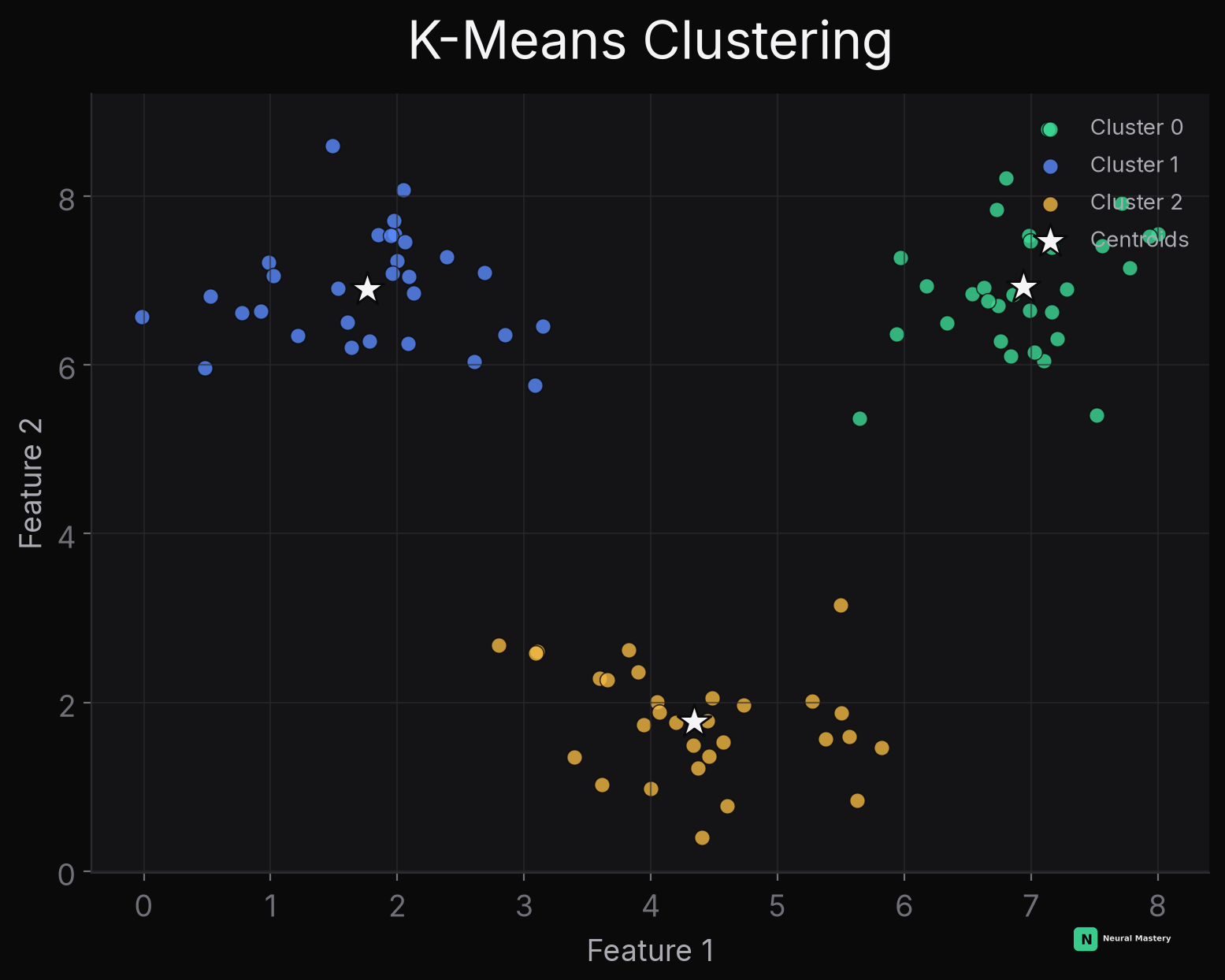
What K-Means is actually optimizing: it minimizes inertia — the total squared distance from each point to its assigned centroid, . This is the unsupervised analog of the squared-error cost function from linear regression — same functional form, just minimized over cluster assignments and centroid positions instead of over a fitted line.
Choosing : since there's no ground truth to check against, use the elbow method — plot inertia against for several candidate values, and look for the point where adding another cluster stops reducing inertia much (a bend in the curve). More rigorous alternatives include the silhouette score, which measures how well-separated clusters actually are.
Click to place your own points (no labels needed — that's the point) and watch real Lloyd's-algorithm assignment/update steps converge live:
Weaknesses:
- Assumes spherical, similarly-sized clusters — because it minimizes distance-to-centroid, K-Means implicitly assumes clusters are round blobs. It fails badly on elongated or non-convex shapes:
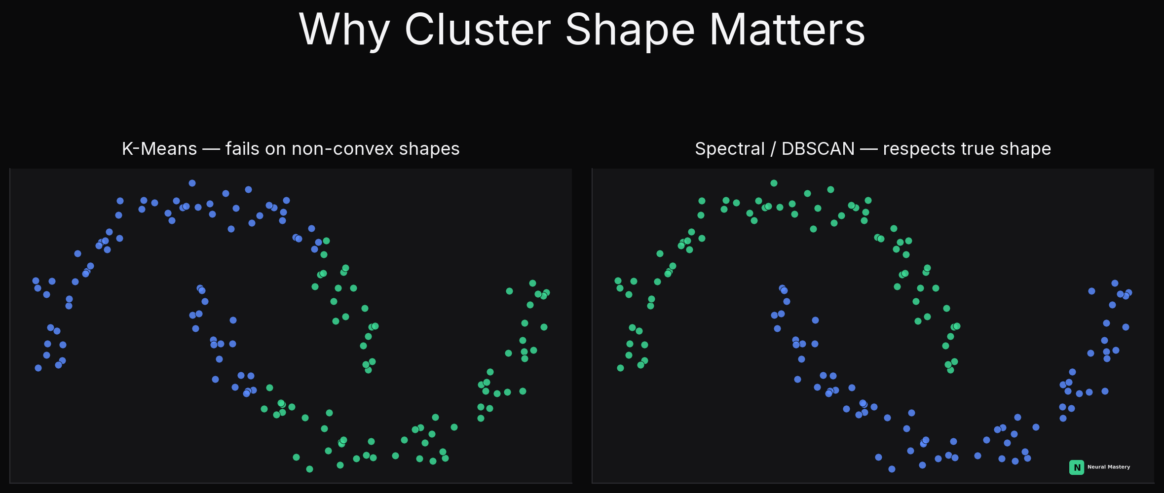
- Sensitive to initialization — a bad random start can converge to a poor local optimum; K-Means++ (a smarter initialization that spreads initial centroids apart) is the standard fix, and the default in most libraries.
- Must choose upfront — unlike hierarchical clustering below.
Try it yourself: implement one K-Means assignment step from scratch, against real test cases.
Hierarchical Clustering
Instead of committing to a fixed , hierarchical clustering builds a full tree of nested groupings, letting you choose how many clusters to cut out after seeing the structure.
Agglomerative (bottom-up, the common approach): start with every point as its own cluster, then repeatedly merge the two closest clusters, until everything is one cluster. The result is a dendrogram:
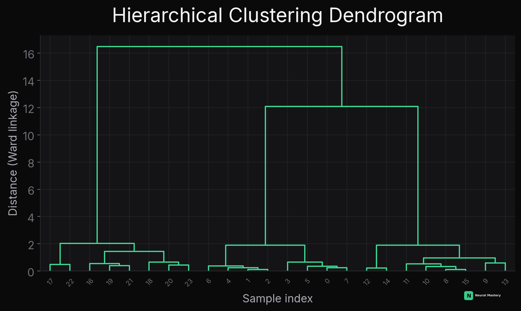
Read the dendrogram like this: the y-axis is the distance at which two groups merged — low merges are confident, tight groupings; high merges are combining already-dissimilar groups. Cutting the tree at any horizontal height gives a specific clustering: cut low for many small, tight clusters; cut high for few, broad clusters. This is hierarchical clustering's key advantage over K-Means — you see the entire range of possible groupings in one structure, and pick the cut that makes sense, rather than committing to one before even looking at the data.
Linkage criteria — how "distance between two clusters" is defined, since a cluster is a group of points, not a single point:
- Single linkage: distance between the two closest points across clusters — can produce long, straggly "chained" clusters.
- Complete linkage: distance between the two farthest points — tends to produce tight, compact clusters.
- Average linkage: average distance between all cross-cluster pairs — a middle ground.
- Ward linkage (used in the dendrogram above): merges whichever pair of clusters increases total within-cluster variance the least — tends to produce well-balanced, similarly-sized clusters, and is the most common default.
Divisive (top-down): the reverse — start with all points in one cluster, and recursively split. Far less common in practice than agglomerative, mainly because deciding how to split optimally at each step is more expensive than deciding what to merge.
K-Means vs. Hierarchical
| K-Means | Hierarchical (Agglomerative) | |
|---|---|---|
| Must choose upfront? | Yes | No — cut the dendrogram anywhere after |
| Scales to large datasets | Yes — roughly per iteration | Poorly — naive implementations are or worse |
| Cluster shape assumption | Spherical/convex | Depends on linkage; still generally struggles with non-convex shapes |
| Deterministic? | No (depends on initialization) | Yes, given a fixed linkage and distance metric |
Next: DBSCAN & HDBSCAN — clustering by density instead of distance-to-centroid, which handles non-convex shapes natively.