PCA, Kernel PCA & Truncated SVD, In Full Depth
Every model so far assumed the given features are the right ones to work with. Dimensionality reduction questions that assumption directly: can most of a dataset's information be captured in far fewer dimensions than it was originally given in?
PCA: Principal Component Analysis
The idea: find the directions in feature space along which the data varies the most, and project onto just those — discarding directions with little variance, since a direction the data barely moves along carries little information.
The mechanism, connecting directly back to Linear Algebra: compute the data's covariance matrix, then find its eigenvectors and eigenvalues. Each eigenvector is a principal component — a direction in the original feature space — and its corresponding eigenvalue is exactly how much variance the data has along that direction. Sort components by eigenvalue (largest first), and keep only the top — that's PCA, in its entirety. Real covariance, real eigendecomposition, real projection:
Choosing : plot each component's share of total variance, and how much accumulates as you keep adding components:
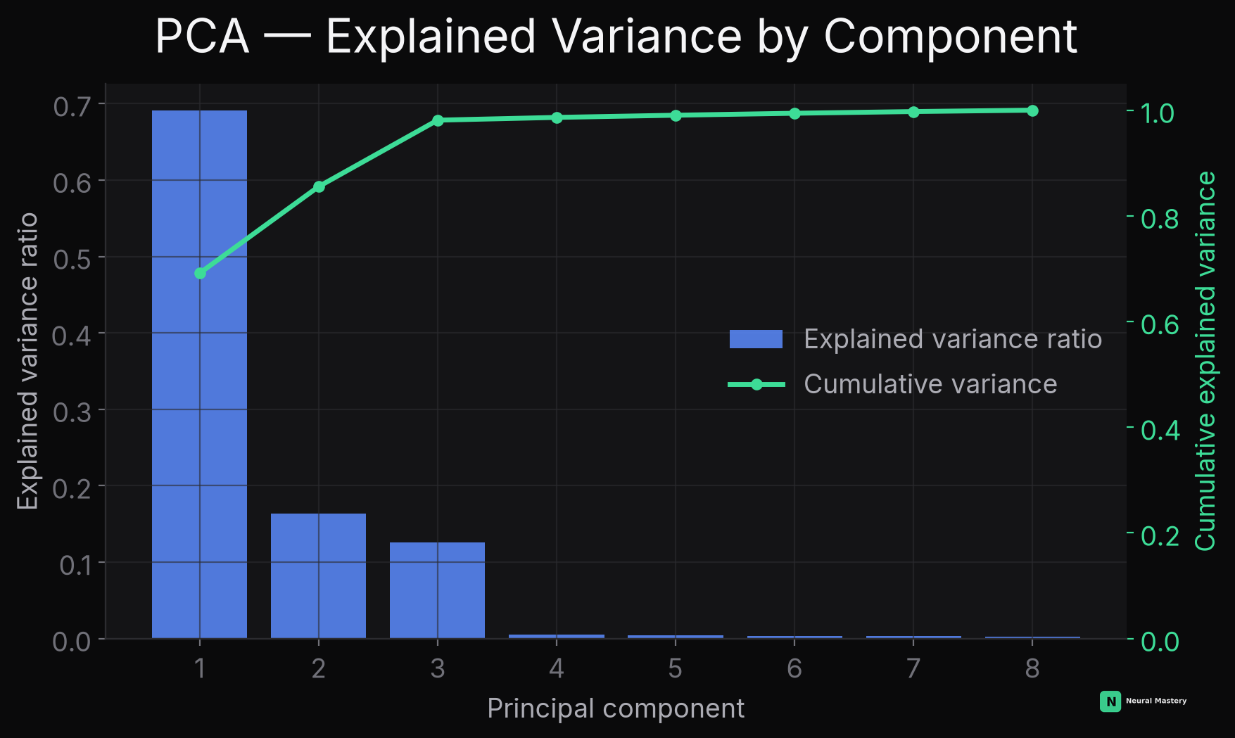
This is a scree plot — look for the "elbow" where additional components stop adding meaningful variance (the same elbow-finding intuition as K-Means' elbow method and DBSCAN's k-distance plot, applied to variance instead). In the chart above, the first 3 components already capture nearly all the variance — the remaining 5 dimensions are mostly noise, exactly matching how this particular synthetic data was generated from 3 underlying latent factors.
Why PCA connects to SVD: the principal components are mathematically identical to the right singular vectors of the (mean-centered) data matrix — PCA and SVD are, in a precise sense, the same computation viewed from two different angles. This is why libraries often compute PCA via SVD directly rather than explicitly forming the covariance matrix — numerically more stable, especially when the number of features is large.
PCA's core limitation: it only captures linear structure — directions that are literally straight lines through feature space. Data that curves (like the two-moons shape) has no good linear projection that preserves its structure.
Kernel PCA
The same kernel trick from SVM, applied to PCA: implicitly map data into a higher-dimensional (possibly infinite-dimensional) space via a kernel function, then perform ordinary PCA in that space — again without ever explicitly computing the high-dimensional mapping, since (exactly as in SVM) the computation only ever needs pairwise kernel evaluations, not the mapped coordinates themselves.
What this buys you: Kernel PCA can capture nonlinear structure that plain PCA misses — e.g. it can successfully separate concentric rings or curved manifolds that are hopeless for linear PCA, using an RBF kernel exactly as described in the SVM page. The tradeoff: choosing the right kernel and its hyperparameters is not automatic, and results are much harder to interpret than plain PCA's direct "variance along an axis" reading.
Truncated SVD
Plain PCA requires mean-centering the data first (subtracting each feature's mean). Truncated SVD skips that step and works directly on the raw data matrix — which matters specifically for sparse data (like a bag-of-words document-term matrix, mostly zeros), where mean-centering would destroy the sparsity and blow up memory usage. Truncated SVD keeps only the top singular values/vectors (see Linear Algebra — SVD) directly, making it the standard dimensionality-reduction tool for text data (this specific application is sometimes called LSA — Latent Semantic Analysis — in the NLP context) and other high-dimensional sparse feature sets.
PCA vs. Kernel PCA vs. Truncated SVD
| PCA | Kernel PCA | Truncated SVD | |
|---|---|---|---|
| Captures nonlinear structure? | No | Yes | No |
| Requires mean-centering? | Yes | Yes (in kernel space) | No |
| Works well on sparse data? | No (centering destroys sparsity) | No | Yes |
| Interpretability | High (variance along axes) | Low | Moderate |
| Typical use | General-purpose linear compression, visualization | Nonlinear structure, moderate data size | Text/sparse feature compression (LSA) |
Next: ICA, t-SNE & UMAP — separating mixed signals, and the nonlinear methods built specifically for visualizing high-dimensional data like embeddings.